Exploring Ordered Sampling in Generative Flow Networks
Ahmed Attia, Idriss Malek, and Salem Lahlou · December 3, 2025
Generative Flow Networks, or GFlowNets, are designed to sample many good solutions rather than return only one optimum. That property is attractive in scientific discovery: if several molecules, structures, or sequences are promising, we want a model that represents all of them [1], [2].
In practice, however, GFlowNets can struggle when rewards are sparse or separated by low-reward regions. Standard on-policy training collects trajectories from the model’s current policy, so an initially weak policy may repeatedly visit an unhelpful part of the state space. This slows learning and can leave reward modes undiscovered.
We investigated a simple intervention: during early training, control the order in which the model sees trajectory lengths. Our main finding is that starting with short trajectories and gradually moving to long ones substantially improves distribution learning in difficult, sparse-reward HyperGrid environments.
A gentle introduction to GFlowNets
A GFlowNet constructs an object through a sequence of actions. The states and allowed transitions form a directed acyclic graph (DAG). A trajectory begins at an initial state, follows edges through the graph, and ends at a terminal state x with non-negative reward R(x).
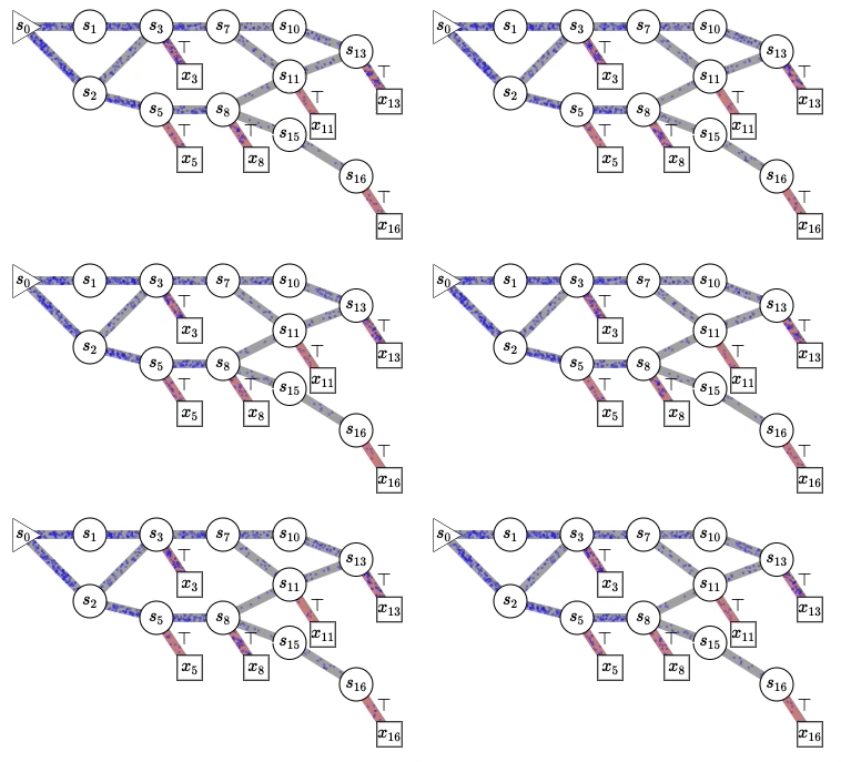
The goal is not to maximize reward in the usual reinforcement-learning sense. Instead, the terminal sampling probability should be proportional to reward:
p(x) = R(x) / Z, where Z = sum of rewards over all terminal states.
This means high-reward objects are sampled more often, while lower-reward objects retain probability mass. The result is a diverse collection that reflects the shape of the reward landscape.
One way to understand GFlowNets is through flows. On a tree, assign each leaf its reward and recursively define the value of an internal state as the sum of its children’s values. Moving to a child in proportion to its value gives the desired terminal distribution. General DAGs are harder because paths can merge and internal states may also terminate. GFlowNets learn a parameterized flow that approximately conserves incoming and outgoing mass at every state while sending terminal flow to rewards.
Training with Trajectory Balance
We use the Trajectory Balance (TB) objective [3]. For a complete trajectory from the initial state to terminal state x, TB compares two quantities:
Z × product of forward probabilities along the trajectory

R(x) × product of backward probabilities along the reversed trajectory
Training minimizes the squared difference between their logarithms. When this balance holds across valid trajectories, the forward policy’s terminal distribution matches R(x) / Z.
A useful property of TB is that the training trajectory does not need to come from the current forward policy. Any behavior distribution with support on valid trajectories can provide training data. This makes TB naturally compatible with off-policy sampling and motivates our curricula.
Why order trajectories by length?
Long trajectories are generally harder: reward must receive credit through more decisions, and the number of possible paths grows. Short trajectories are easier but cover less of the graph.
Curriculum learning usually presents easier examples before harder ones [4]. Topological Experience Replay suggests another direction: use the topology of the experience graph to propagate values backward from rewarding states, encouraging broader early coverage [5]. These views lead to two opposite schedules:
- Small-then-Large (STL): begin with short, lower-entropy trajectories, then increase their length. This is the conventional easy-to-hard curriculum and is intended to establish reliable credit assignment before adding complexity.
- Large-then-Small (LTS): begin with long trajectories, then decrease their length. Inspired by topological replay and dynamic programming, this schedule aims to propagate reward information broadly through the DAG before refining shorter paths.
The two methods change only the early data-collection schedule. They use the same model and the same TB loss as the baseline.
Length-conditioned sampling
We maintain a target trajectory length between L_min and L_max. To construct a batch for target length L:
- Start each trajectory at the root state.
- Mask the Exit action while the current step is less than
L. - Sample the remaining actions from the forward policy.
- At step
L, force Exit if the trajectory has not already terminated. - Apply the ordinary TB update to the completed batch.
This procedure produces valid trajectories of the requested length while leaving the learning objective unchanged.
The curriculum schedule
Only the first 10% of training uses length conditioning. If the complete run contains N iterations, the curriculum receives floor(0.10 × N) iterations. We divide these iterations approximately uniformly among all target lengths; any remainder goes to the earliest stages.
STL traverses lengths in ascending order:
L_min, L_min + 1, ..., L_max
LTS uses the reverse order:
L_max, L_max - 1, ..., L_min
After this initial phase, both methods spend the remaining 90% of training on standard on-policy TB updates. We do not use an experience replay buffer.
Experimental setup
We evaluated the schedules on HyperGrid, a synthetic discrete DAG whose reward sparsity can be controlled. It is useful here because it lets us systematically make exploration harder while retaining the exact ground-truth terminal distribution.
We tested five (height, dimension) configurations:
| Height | Dimensions |
|---|---|
| 32 | 3 |
| 32 | 4 |
| 64 | 2 |
| 64 | 3 |
| 128 | 2 |
For every configuration, we compared standard on-policy TB, STL, and LTS. We swept the background reward R0, kept R1 = 1 and R2 = 3, and measured the L1 distance between the learned and ground-truth terminal distributions. Lower distance is better.
Every method used the same optimizer and training budget. Each update consumed a batch of 16 trajectories, and a complete run consumed 200,000 trajectories. The forward policy was a two-layer MLP with hidden size 256. The backward policy was fixed to be uniform over parent states. We implemented the experiments with TorchGFN [6] and ran them on a MacBook Air M4.
Results
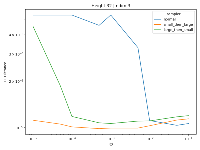
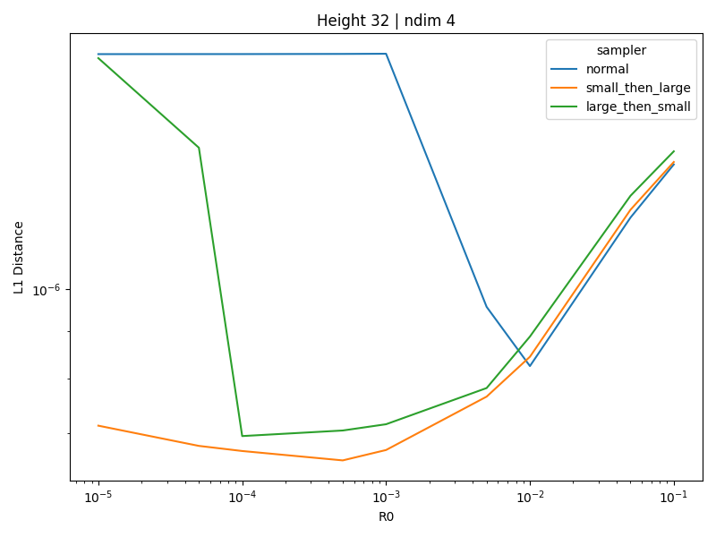
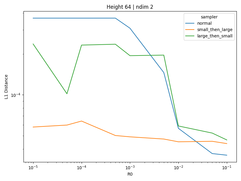
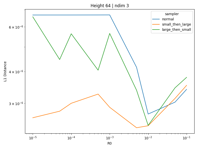
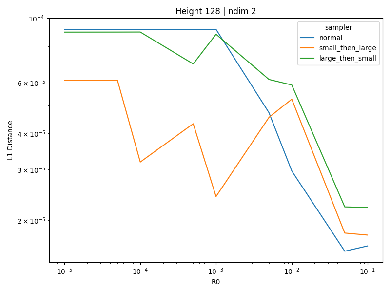
Across all five configurations, the same pattern emerged:
- STL was best in the hardest reward settings. When
R0was small, samplers had to cross a low-reward valley to recover all reward modes. STL consistently achieved the lowest L1 distance. - LTS was generally between STL and the baseline. Prioritizing long trajectories helped early coverage, but it was less effective than building from short trajectories.
- The baseline caught up when rewards became denser. Once
R0rose beyond roughly10^-2, ordinary on-policy sampling recovered the modes efficiently and matched STL. LTS remained weaker in this regime.
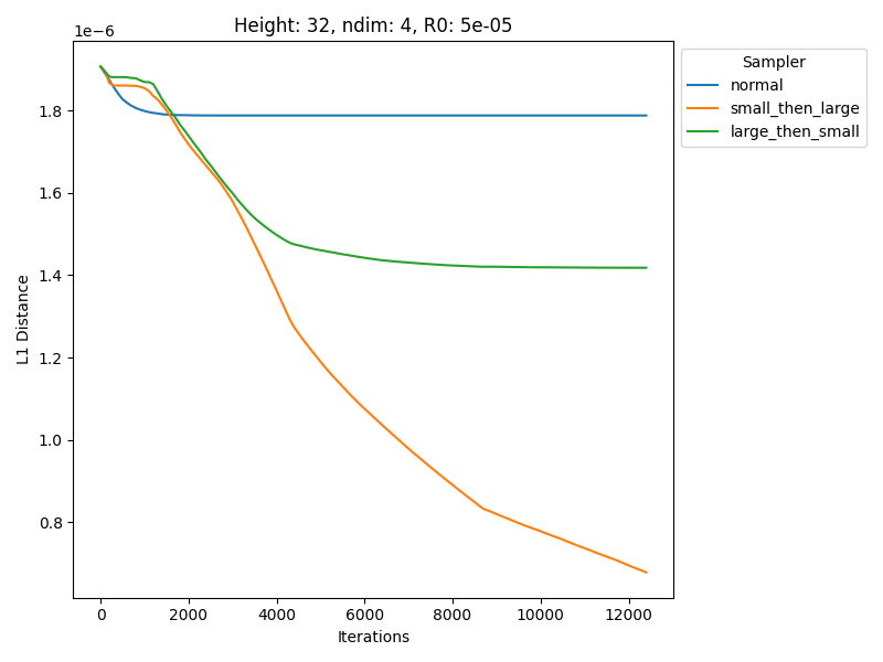
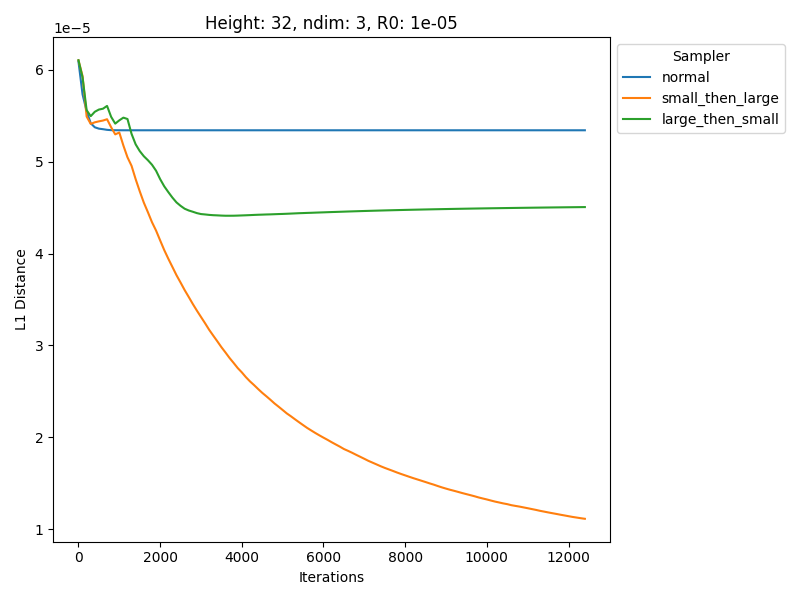
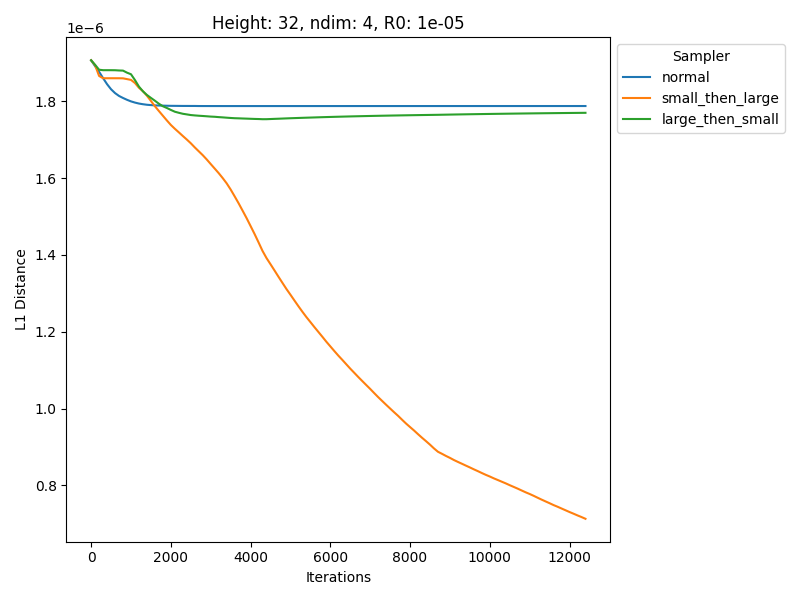
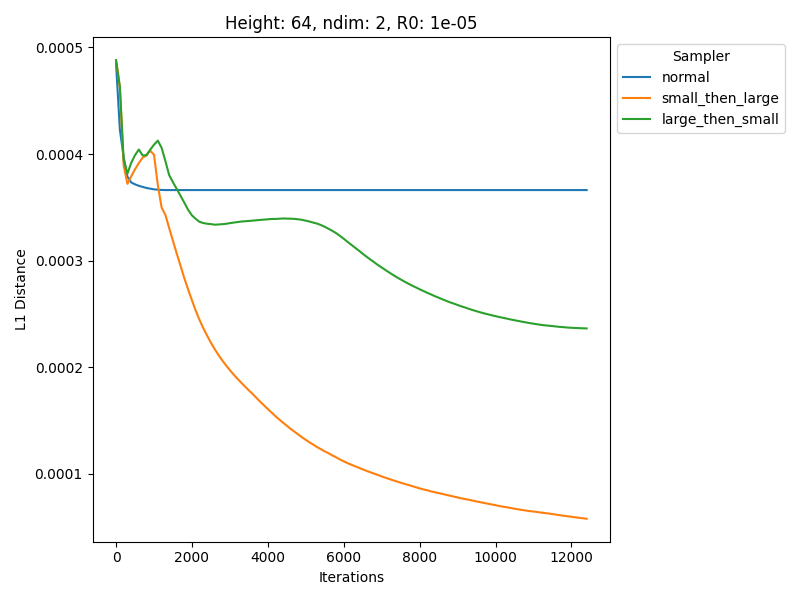
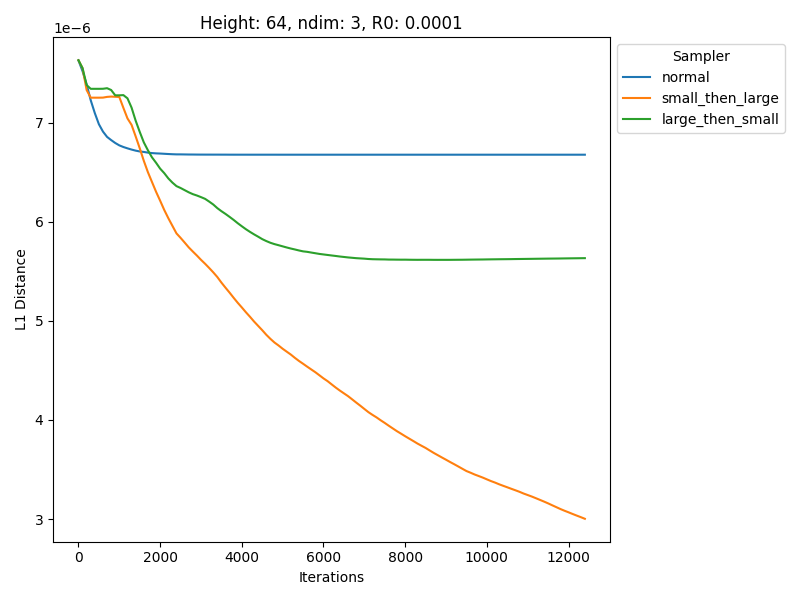
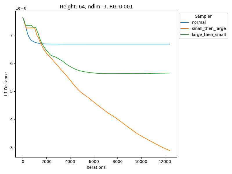
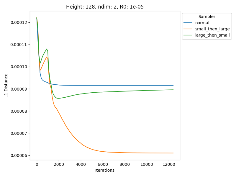
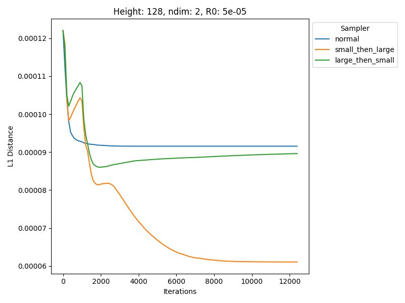
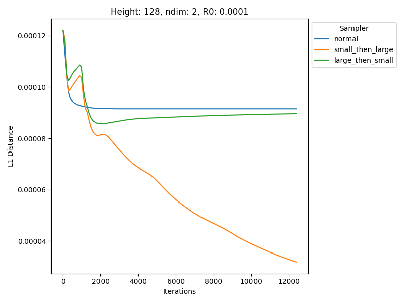
The learning curves support the same interpretation. STL continued to find better solutions and explore the environment in cases where the other samplers plateaued. The benefit is therefore concentrated where exploration and early credit assignment are genuinely difficult; the curriculum is not necessary when the reward already provides a strong learning signal.
Extended learning curves
The plots below show L1 distance throughout training for nine representative runs. They make the optimization behavior visible rather than showing only the final error: STL frequently descends earlier or continues improving after the alternatives flatten out.
The curricula in motion
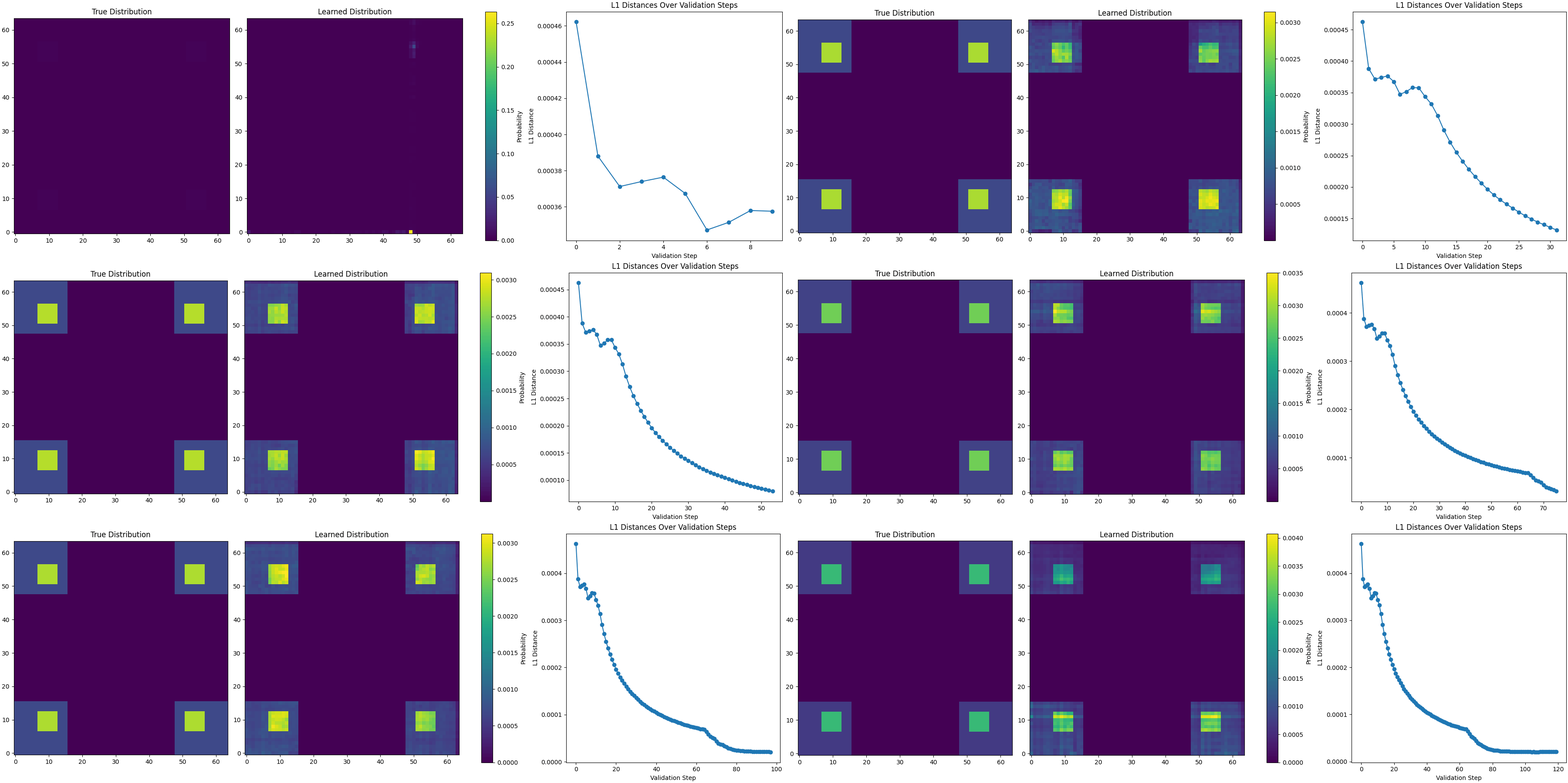
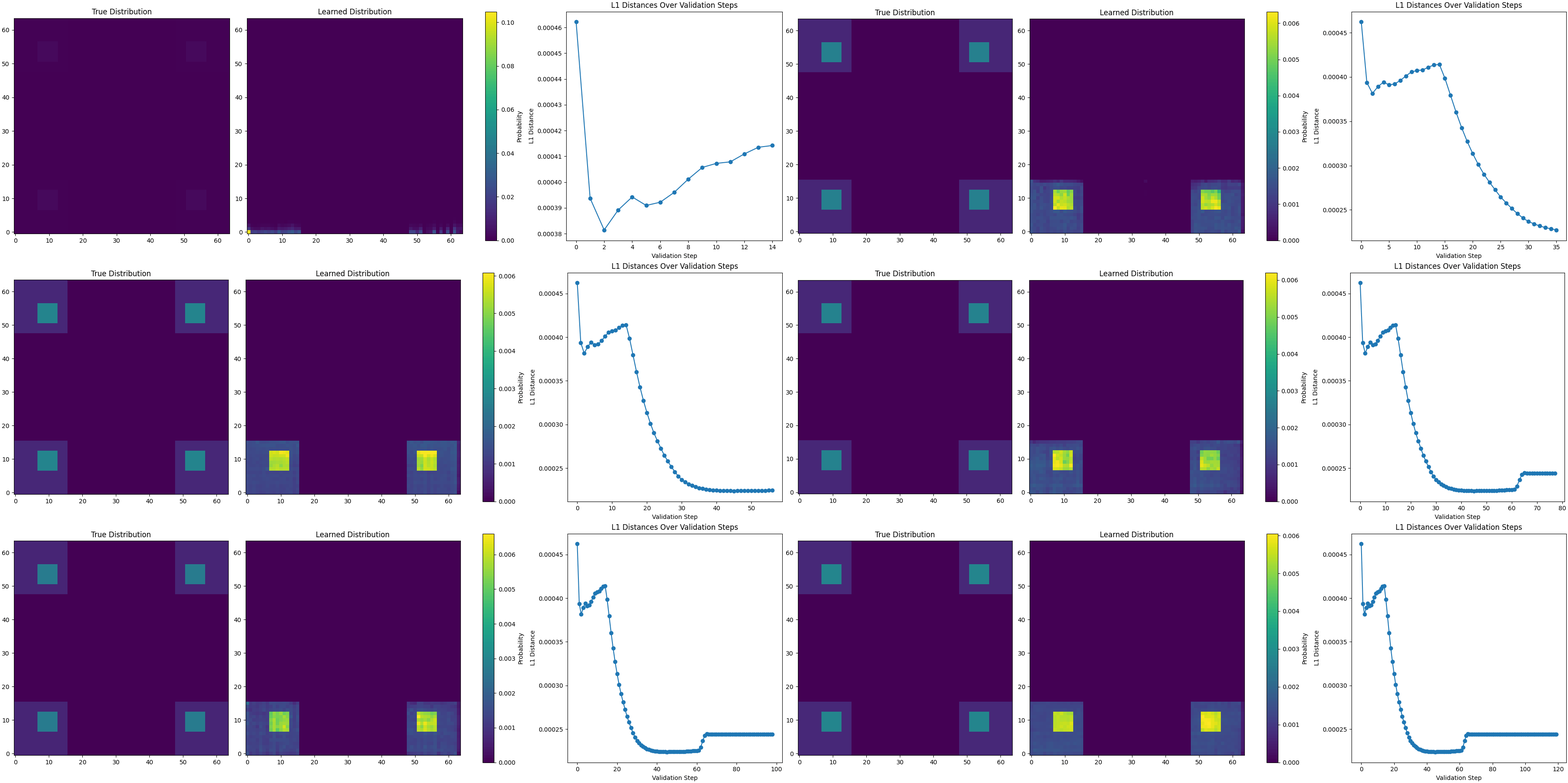
The animations pair the evolving learned distribution with its target and L1 distance. STL grows from short trajectories toward longer ones, while LTS runs the same curriculum in reverse. It’s evident that STL converges more quickly, finds all the modes, and achieves a lower final L1 distance.
What we learned
The experiments suggest that trajectory length is a useful control variable for early GFlowNet training. An easy-to-hard ordering gives the model short credit-assignment problems first, then expands the portion of the state graph it must handle. This improved sample efficiency and mode coverage without changing the model architecture or objective.
The hard-to-easy alternative was still useful in some sparse settings, supporting the broader idea that topology-aware sampling can improve exploration. But its weaker performance also shows that broad coverage alone is not enough: the model benefits more from first learning a stable local foundation.
Limitations and next steps
These findings are preliminary. Our evaluation is confined to HyperGrid, a synthetic discrete DAG, and does not yet establish that the same gains transfer to molecule generation or other real scientific tasks. Trajectory length is also a coarse proxy for difficulty: two trajectories of equal length can differ substantially in reward, branching structure, or uncertainty.
The schedule is fixed and uniform. It does not react to the model’s learning progress, and we currently lack a convergence or variance analysis for these non-stationary off-policy curricula, particularly STL.
Natural next steps are to:
- learn an adaptive curriculum instead of fixing the order in advance;
- combine length with reward, uncertainty, or graph-topology signals;
- study convergence and gradient variance under changing behavior distributions;
- test on larger domains such as synthesizable molecule generation.
Conclusion
We introduced two simple off-policy curricula for GFlowNets. Small-then-Large begins with short trajectories and increases their length; Large-then-Small does the reverse to encourage broad early propagation. In sparse-reward HyperGrids, STL consistently learned the target distribution more accurately than standard on-policy training and LTS. When rewards were easier to discover, the baseline caught up.
The central lesson is simple: exploration depends not only on where a generative policy goes, but also on when it learns to go there.
References
- Bengio, Y., Lahlou, S., Deleu, T., Hu, E. J., Tiwari, M., and Bengio, E. “GFlowNet Foundations.” 2021.
- Jain, M., Deleu, T., Hartford, J., Liu, C.-H., Hernandez-Garcia, A., and Bengio, Y. “GFlowNets for AI-Driven Scientific Discovery.” Digital Discovery, 2023.
- Malkin, N., Jain, M., Bengio, E., Sun, C., and Bengio, Y. “Trajectory Balance: Improved Credit Assignment in GFlowNets.” NeurIPS, 2022.
- Bengio, Y., Louradour, J., Collobert, R., and Weston, J. “Curriculum Learning.” ICML, 2009.
- Hong, Z.-W., Chen, T., Lin, Y.-C., Pajarinen, J., and Agrawal, P. “Topological Experience Replay.” 2023.
- Lahlou, S., Viviano, J. D., Schmidt, V., and Bengio, Y. “TorchGFN: A PyTorch GFlowNet Library.” 2023.
- Mila. “The GFlowNet Tutorial.”
If you have questions or would like to discuss extensions of this work, feel free to email me.